Antoine's Blog

In this post, I'll dive into a comparison of two popular machine learning models: Random Forest and Boosted Trees (XGBoost). I will use a dataset from a study on cockle densities in relation to green macroalgal (GMA) biomass in Yaquina Bay, Oregon. By analyzing their performance on this dataset, we'll explore which model is better suited for this type of ecological data.

Credit: Yakfish Taco

Introduction to Random Forest and Boosted Trees

Random Forest and Boosted Trees (XGBoost) are two ensemble learning methods widely used in machine learning for classification and regression tasks. Random Forest operates by constructing a multitude of decision trees during training and outputs the class that is the majority vote of the individual trees. This approach helps in reducing overfitting and improving model accuracy by averaging the predictions from multiple trees. On the other hand, Boosted Trees, particularly XGBoost, enhance predictive performance through a technique called boosting. XGBoost builds trees sequentially, where each new tree corrects errors made by the previous ones, and it optimizes model performance by focusing on difficult-to-predict instances. Both methods leverage the strength of ensemble learning but differ in their approach to aggregating predictions, making them suitable for various types of data and problem domains.

Credit: Janusz Szwabiński

Dataset Overview

The dataset, originally collected during field surveys in June and August 2014, includes various attributes like site, station, survey date, presence of cockles, and environmental factors such as water depth and algal coverage. The target variable, Present, indicates whether cockles were observed in the sampled area.

Preprocessing and Modeling Steps

Let's go through the steps in the Python script used to preprocess the data and train the models.

1. Loading and formatting the Dataset:

   file_path = './cockle-fieldsurveydata-xlsx-1.xls'
   df = pd.read_excel(file_path, 'Data')
   df.dropna(inplace=True)
   
   % Date parsing
   df['Date'] = pd.to_datetime(df['Date'], format='%m/%d/%Y') 
   
   for col in ['Easting', 'Shallow_cm', 'Deep_cm', 'Avg_cm']:
    df[col] = df[col].astype(str).str.replace(',', '.').astype(float)
   
   for column in df.select_dtypes(include=['object']).columns:
    df[column] = LabelEncoder().fit_transform(df[column])
      
   % Feature Selection
   X = df.drop(['Uncovered', 'Semi_covered', 'Buried', 'Total','Present','Site','Station','Easting'], axis=1)
   y = df['Present']
    
   % Data splitting
   X_train, X_test, y_train, y_test = train_test_split(X, y, test_size=0.2, random_state=42)
   

The features for the model (X) were selected by excluding irrelevant or redundant columns, while the target variable (y) was set to the Present column (which is a binary indicator equivalent to Total>0). Finally, the data was split into training and testing sets, with 80% of the data used for training and 20% reserved for testing.

Justification for Removing Localization Variables

In the context of this analysis, the localization variables such as Site, Station, and Easting were removed during the feature selection process. These variables represent spatial information about the specific locations where samples were collected.

Including these variables could lead to overfitting, where the model learns to associate specific locations with outcomes rather than general patterns that can be applied to new, unseen data. By removing these localization variables, we ensure that the model focuses on ecological and environmental features that are more likely to provide generalizable insights into cockle presence.

2. Training the Models:

   % Random Forest
   rf_model = RandomForestClassifier(n_estimators=100, random_state=42)
   rf_model.fit(X_train, y_train)
   rf_predictions = rf_model.predict(X_test)
   
   % Boosted Trees (XGBoost)
   xgb_model = XGBClassifier(use_label_encoder=False, eval_metric='logloss', random_state=42)
   xgb_model.fit(X_train, y_train)
   xgb_predictions = xgb_model.predict(X_test)
   

The Random Forest model was trained with 100 trees, and predictions were made on the test set. The XGBoost model was trained with default settings, and predictions were made similarly.

Performance Comparison and Results

After training both the Random Forest and Boosted Trees (XGBoost) models on the dataset, we evaluated their performance using several metrics, including accuracy, precision, recall, F1-score, confusion matrices, and ROC AUC scores.

Accuracy

• Random Forest Accuracy: 0.54
• Boosted Trees (XGBoost) Accuracy: 0.50

Accuracy measures the proportion of correct predictions made by the model. In this case, the Random Forest model slightly outperformed XGBoost, achieving an accuracy of 54% compared to XGBoost’s 50%.

Classification Reports

Random Forest Classification Report:

               precision    recall  f1-score   support

           0       0.55      0.50      0.52        12
           1       0.54      0.58      0.56        12

    accuracy                           0.54        24
   macro avg       0.54      0.54      0.54        24
weighted avg       0.54      0.54      0.54        24

Boosted Trees (XGBoost) Classification Report:

               precision    recall  f1-score   support

           0       0.50      0.42      0.45        12
           1       0.50      0.58      0.54        12

    accuracy                           0.50        24
   macro avg       0.50      0.50      0.50        24
weighted avg       0.50      0.50      0.50        24

From the classification reports, we see that the Random Forest model has a slightly better balance between precision and recall, especially for class 1 (Presence). The F1-scores, which balance precision and recall, show that Random Forest provides a better overall performance with an F1-score of 0.56 for class 1 compared to 0.54 for XGBoost.

Confusion Matrices

Random Forest Confusion Matrix:

   [[6 6]
    [5 7]]

Boosted Trees (XGBoost) Confusion Matrix:

   [[5 7]
    [5 7]]

The confusion matrices reveal how well each model distinguishes between the two classes (0 and 1, or Absence and Presence of cockles). Both models show a similar pattern, with Random Forest slightly better at correctly predicting class 1.

ROC AUC Scores

• Random Forest ROC AUC Score: 0.517
• Boosted Trees (XGBoost) ROC AUC Score: 0.594

The ROC AUC score is a measure of the model’s ability to distinguish between classes across all classification thresholds. Here, XGBoost has a higher ROC AUC score (0.594) compared to Random Forest (0.517), indicating that XGBoost has a better overall ability to separate the two classes, despite its lower accuracy.

Feature Importance Analysis

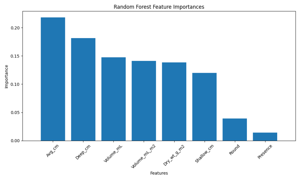
Understanding feature importance is pivotal for interpreting machine learning models, as it reveals which attributes are most influential in predictions. In our analysis of the Random Forest and Boosted Trees (XGBoost) models, we examined how each algorithm evaluates feature importance.

Random Forest determines feature importance by averaging the decrease in impurity across all trees, providing a straightforward measure of how each feature contributes to model accuracy. The resulting feature importance plot highlights key features that significantly influence predictions. The three most important features for the Random Forest model are the mean depth and the deepest depth of the apparent redox potential discontinuity within a subsampled corner of the quadrat, and the volume of wet GMA.

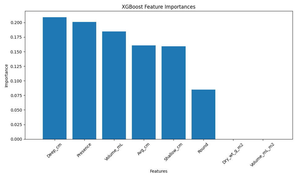
Conversely, XGBoost assesses feature importance based on the gain, which reflects the improvement in model accuracy attributed to each feature. This method can unveil different insights, as XGBoost builds trees sequentially, capturing complex interactions between features. The three most important features for the XGBoost model are the deepest depth of the apparent redox potential discontinuity within a subsampled corner of the quadrat, the GMA presence (binary variable) and the volume of wet GMA.

Conclusion

In summary, while Random Forest achieved slightly higher accuracy and better-balanced classification metrics, XGBoost demonstrated superior performance in terms of ROC AUC score. This suggests that XGBoost might be more robust in identifying the presence of cockles across varying thresholds, making it a valuable model depending on the specific goals of the analysis.

My Python code for this project is available on my GitHub repository. Feel free to check it out here.

Source

The dataset has been found on data.world. It is associated with the following publication: Lewis, N., and T. DeWitt. Effect of Green Macroalgal Blooms on the Behavior, Growth, and Survival of Cockles (Clinocardium nuttallii) in Pacific NW Estuaries. MARINE ECOLOGY PROGRESS SERIES. Inter-Research, Luhe, GERMANY, 582: 105-120, (2017).

In various scientific and engineering applications, there is a need to optimally arrange objects within a given space. One fascinating instance is the problem of placing multiple circles within a rectangular area to maximize the covered area without overlapping. This task is highly relevant in experiment design. In this post, I explore a Python-based approach using the Pyomo optimization library to solve this problem.

Background

The circle placement problem can be categorized as a type of packing problem, which is a well-known challenge in operations research and combinatorial optimization. The primary objective is to arrange a set of circles within a bounded area such that the total covered area is maximized and no circles overlap.

Why This Is Useful

Optimal placement of objects is crucial in many fields:

• Experiment Design: Efficient use of space can lead to better experiment setups and resource utilization.
• Manufacturing: In industries, optimizing the layout of components can minimize waste and reduce costs.
• Urban Planning: Placing structures optimally in a given area ensures better space utilization and accessibility.

The Python Code

The Python script that uses Pyomo, a popular optimization library, to solve the circle placement problem is available on my Github. The code creates a model, defines constraints to prevent overlapping, and ensures circles stay within the boundaries. The solution is obtained by testing multiple initializations to find the best arrangement.

Explanation of the Code

Defining the Area and Parameters:

• The area dimensions are defined using AREA_WIDTH and AREA_HEIGHT.
• The number of circles (NUM_CIRCLES) and the number of initializations to test (NUM_INITIALIZATIONS) are set.

Creating the Model:

• The create_model() function defines the Pyomo model.
• Variables x, y, and r represent the x-coordinate, y-coordinate, and radius of each circle, respectively.
• The objective is to maximize the total area covered by the circles.
• Constraints are added to prevent overlap and ensure that circles stay within the defined area.

Solving the Model:

• The solve_model() function uses the IPOPT solver to solve the model.
• Multiple initializations are tested to find the best solution.

Calculating Coverage and Visualization:

• The best solution is selected based on the maximum covered area.
• The coverage percentage is calculated and displayed.
• The final positions of the circles are plotted using Matplotlib.

Results

An example output from running the code might look like this:

Coverage rate: 85.91% I'm still far from this solution! It's important to note that due to the complexity of the circle packing problem, the solution found may not always be fully optimized. Different initializations and solvers can yield varying results. On this example there is still a lot of space on the right hand corners.

Conclusion

This Pyomo-based approach provides a powerful method to tackle the circle packing problem efficiently. By leveraging optimization techniques, it ensures that circles are placed optimally within a defined area, maximizing the area covered while adhering to specified constraints. Such techniques are really pertinent in experiment design, logistics planning, and other domains where efficient space utilization is crucial.

For further exploration:

• Pyomo Documentation: Pyomo
• IPOPT Solver Documentation: IPOPT
• inspiration: yetanothermathprogrammingconsultant

In this post, I'll walk through a Python web application that fetches detailed information about fish species from FishBase, and then summarizes the data using OpenAI's GPT-3.5 model. This application is built using the Flask framework and includes web scraping and natural language processing.

Setting Up Flask

First, we import the necessary libraries and set up our Flask application:

from flask import Flask, request, jsonify, render_template
import requests
from bs4 import BeautifulSoup
from openai import OpenAI
import wikipediaapi

app = Flask(__name__)

Fetching Fish Information from FishBase

The get_fish_info function takes the species name as input, constructs the URL for FishBase, and scrapes the information using BeautifulSoup:

def get_fish_info(species):
    url = f'https://www.fishbase.se/summary/{species}'
    response = requests.get(url)
    
    if response.status_code != 200:
        return {"error": "Species not found or failed to fetch data"}
    
    soup = BeautifulSoup(response.content, 'html.parser')
    [s.extract() for s in soup(['style', 'script', '[document]', 'head', 'title'])]
    info_fishbase = soup.getText()
    
    return {
         "info": info_fishbase,
    }

Summarizing the Information with OpenAI GPT-3.5

To provide a concise summary of the fetched data, I use OpenAI's GPT-3.5. The generate_summary function interacts with the OpenAI API to generate the summary:

def generate_summary(info):
    api_key = 'YOUR_OPENAI_API_KEY'  # Replace with your actual OpenAI API key
    client = OpenAI(api_key=api_key)
    
    prompt = f"Generate a concise summary for the following fish information:\n\n{info}. The summary must contain all the important features and data about the species, based on the information given."

    completion = client.completions.create(
        model="gpt-3.5-turbo-instruct",
        prompt=prompt,
        max_tokens=150
    )
    return completion.choices[0].text.strip()

Creating Routes in Flask

I define two routes: one for the home page and another for fetching the fish information:

@app.route('/')
def index():
    return render_template('index.html')

@app.route('/fetch', methods=['POST'])
def fetch():
    data = request.json
    species = data['species'].replace(' ', '-')
    
    fish_info = get_fish_info(species)
    if 'error' in fish_info:
        return jsonify(fish_info), 404

    summary = generate_summary(fish_info['info'])
    fish_info['summary'] = summary

    return jsonify(fish_info)

Running the Application

Finally, we run the Flask application in debug mode:

if __name__ == '__main__':
    app.run(debug=True)

From that, I build a simple web app (the whole project is available on my github ):

The length of the summary is determined by the number of tokens allowed in the model's response. In this example, the token limit caused the last sentence to be incomplete.

Open Fisheries is a platform that compiles global fishery data, offering records of global fish capture landings from 1950 onwards. I have converted the great work from the rfisheries R package to Python to facilitate data analysis.

You can use the API to gather the total fish capture landings for a specific country. For example, the following chart shows the total landings for Canada:

The API can also be used to gather the total fish capture landings for different species. In this example, we look at the total landings for three species: Dentex dentex (DEC), Dentex congoensis (DNC), and Dentex macrophtalmus (DEL):

As an illustrative example, I focused on species that are assessed globally and present in France, which can be accessed here.

To better understand the conservation status of these species, I grouped them according to their IUCN status. The IUCN Red List categorizes species based on their risk of extinction, helping to guide conservation efforts. The statuses range from Least Concern to Critically Endangered, providing a critical framework for assessing biodiversity.

The IUCN red list status are:

Calling the Open Fisheries API, I was able to retrieve catch trends of species based on their conservation status, highlighting the need for targeted management and conservation strategies.

Here is a visual representation of the catch data by IUCN status:

To continue this work, I am looking for data on global fishing intensities, which would enable the calculation of Maximum Sustainable Yield (MSY) and other key statistics for more effective fisheries management. Unfortunately, I haven't been able to find this data (maybe I should look to Ray Hilborn's global fisheries database). Its availability would significantly bolster my analysis.

My Python code for this project is available on my GitHub repository. Feel free to check it out here.

As I was gaining experience in machine learning, I found myself tumbling down a rabbit hole centered around Convolutional Neural Networks (CNNs). In particular, I was game to experiment with these networks onto spatial patterns. I stumbled upon the MovingPandas library for movement data and analysis, which provided incredibly intuitive tutorials. I focused my attention to the example using AIS data published by the Danish Maritime Authority on the 5th July 2017 near Gothenburg.

It was a good start to apply some CNN. Inspired by the work of Chen et al. (2020) who train neural network to learn from labeled AIS data, I set out a CNN aiming at classifying ships by their categories, given their trajectory. For now, this is not completely functionnal since the dataset is really restricted. However the method is scalable.

First, I designed a streamlit webapp (the code is available on my github) to display vessels trajectories and densities given their category.

I removed categories of vessel without enough sample. I also filtered out trajectories which duration is less than half the median duration.

To train the CNN I need to compute images from the trajectories. There will be image of 128x128 pixels. I split trajectories in segments of half the median duration (~9h). I browse these segments and for each step of time, I fill the corresponding pixel (by mapping the matrix of pixels to the min/max longitude and latitude available in the data). I discard all the motionless trajectories.

Once I have all the images, I set up my CNN:

model = tf.keras.Sequential([
tf.keras.layers.Conv2D(32, (3, 3), activation='relu', input_shape=(128, 128, 3)),
tf.keras.layers.MaxPooling2D(2, 2),
tf.keras.layers.Conv2D(64, (3, 3), activation='relu'),
tf.keras.layers.MaxPooling2D(2, 2),
tf.keras.layers.Conv2D(128, (3, 3), activation='relu'),
tf.keras.layers.MaxPooling2D(2, 2),
tf.keras.layers.Flatten(),
tf.keras.layers.Dense(512, activation='relu'),
tf.keras.layers.Dense(num_classes, activation='softmax')  # Use num_classes for the output layer ])

This is a classical architecture of a CNN network, composed of an alternation of convolution layers (feature identification) and pooling layers (dimension reduction). You'll find a good summary of pooling layers here .

Then, I compile the model and fit the model :

model.compile(optimizer='adam',
   loss='categorical_crossentropy',  # Use 'categorical_crossentropy' for multi-class classification
   metrics=['accuracy'])

history = model.fit(
   train_generator,
   steps_per_epoch=train_generator.samples // train_generator.batch_size,
   epochs=10
 )

Unfortunately my dataset was not big enough to give accurate statistics. The model seems able to recognize some patterns:

This model may be improved by encoding acceleration and speed in the color channels. Also, I should use data augmentation techniques (rotations?) to populate the dataset.