Antoine's Blog

What is Stacking?

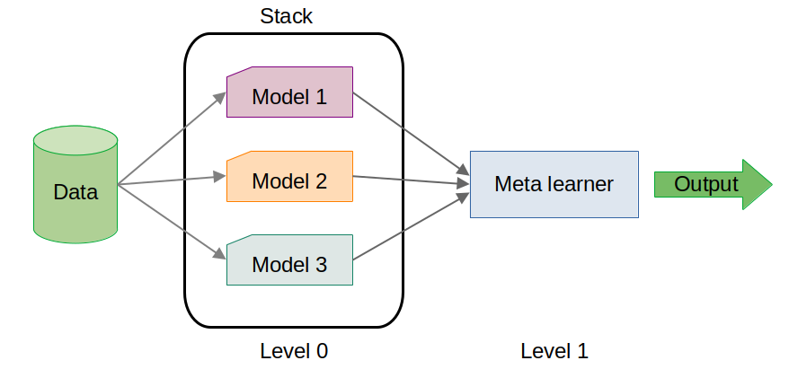
Stacking is an ensemble learning technique that combines the predictions of multiple base models (level 0 models) to generate a final prediction using a meta-model (level 1 model). Unlike simple voting or averaging methods, stacking uses a meta-model to learn how to best combine the predictions of base models, thereby capturing complex patterns and relationships in the data.

How Stacking Works:

1. Base Models (Level 0 Models): These are the individual models that are trained on the same dataset. They could be of different types, such as a decision tree, a k-nearest neighbors model, or a support vector machine.

2. Meta-Model (Level 1 Model): The predictions of the base models are used as features to train a meta-model. This model learns the optimal way to combine the base models' predictions to improve accuracy.

3. Final Prediction: The meta-model produces the final prediction by integrating the predictions of the base models.

Why using Stacking?

• Improved Performance: By combining multiple models, stacking can often outperform any single model. It leverages the strengths of each base model while mitigating their weaknesses.

• Flexibility: Stacking allows you to combine different types of models, making it versatile for various datasets and problems.

• Reduced Overfitting: The meta-model can learn to generalize better by combining the predictions of overfitted base models, leading to a more robust final model.

The main drawback of Stacking is the training time. It’s computationally expensive and time-consuming, especially for large datasets.

Practical Example: Stacking in Action - Predicting Poisonous Mushrooms on Kaggle

For this practical example, we'll walk through how I used stacking to participate in the Kaggle competition Playground Series - Season 4, Episode 8: Binary Prediction of Poisonous Mushrooms. The goal of the competition is to predict whether a mushroom is edible or poisonous based on its physical characteristics.

I'll skip the loading and pre-processing parts that you can find in my jupyter notebook.

Once the data are correctly formatted, I trained three different models as the base learners:

from sklearn.ensemble import RandomForestClassifier, GradientBoostingClassifier
from sklearn.neighbors import KNeighborsClassifier
from sklearn.linear_model import LogisticRegression

# Initialize classifiers
rf = RandomForestClassifier(n_estimators=100, random_state=42, n_jobs = -1)
gb = GradientBoostingClassifier(n_estimators=100, random_state=42)
knn = KNeighborsClassifier(n_neighbors=5)

# Train classifiers
rf.fit(X_TRAIN, Y_TRAIN)
gb.fit(X_TRAIN, Y_TRAIN)
knn.fit(X_TRAIN, Y_TRAIN)

# Predict on the validation set
y_pred_rf = rf.predict(X_VAL)
y_pred_gb = gb.predict(X_VAL)
y_pred_knn = knn.predict(X_VAL)

To enhance the prediction accuracy, I combined these base models using a stacking approach:

from sklearn.ensemble import StackingClassifier
# Define base learners
base_learners = [
    ('rf', rf),
    ('gb', gb),
    ('knn', knn)
]

# Define meta-learner
meta_learner = LogisticRegression()

# Initialize Stacking Classifier
stacking_clf = StackingClassifier(estimators=base_learners, final_estimator=meta_learner)

# Train Stacking Classifier
stacking_clf.fit(X_TRAIN, y_train)

# Predict on validation set
y_pred_stacking = stacking_clf.predict(X_VAL)

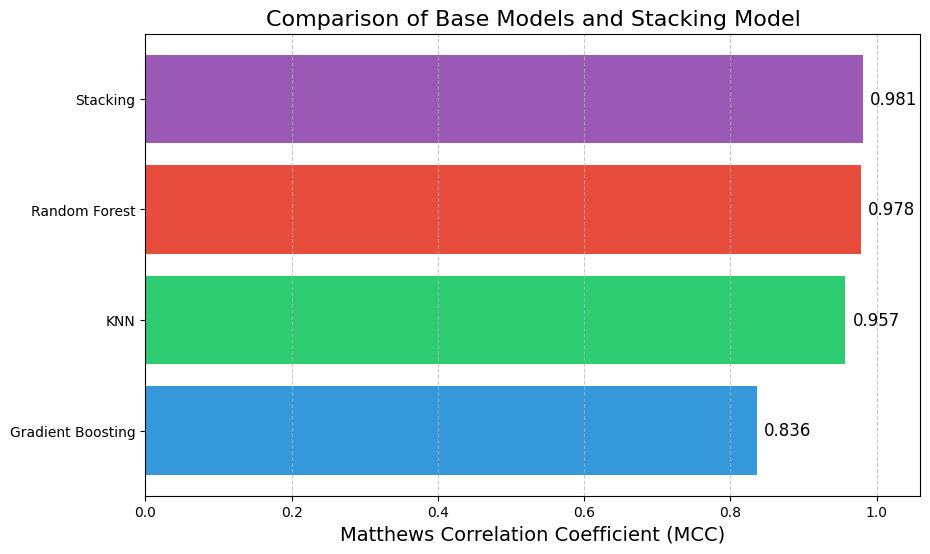
Finally, I evaluated the performance of each base model and the stacked model on the validation set to see the benefits of stacking:

from sklearn.metrics import matthews_corrcoef

# Calculate mcc for each model
mcc = {
    'Random Forest': matthews_corrcoef(Y_VAL, y_pred_rf),
    'Gradient Boosting': matthews_corrcoef(Y_VAL, y_pred_gb),
    'KNN': matthews_corrcoef(Y_VAL, y_pred_knn),
    'Stacking': matthews_corrcoef(Y_VAL, y_pred_stacking)
}


# Sort MCC values for better visualization
sorted_mcc = dict(sorted(mcc.items(), key=lambda item: item[1]))

# Plot the MCCs
plt.figure(figsize=(10, 6))
bars = plt.barh(list(sorted_mcc.keys()), list(sorted_mcc.values()), color=['#3498db', '#2ecc71', '#e74c3c', '#9b59b6'])

# Add MCC values to the bars
for bar in bars:
    plt.text(bar.get_width() + 0.01, bar.get_y() + bar.get_height()/2, 
             f'{bar.get_width():.3f}', va='center', fontsize=12)

plt.xlabel('Matthews Correlation Coefficient (MCC)', fontsize=14)
plt.title('Comparison of Base Models and Stacking Model', fontsize=16)
plt.xlim([0., 1.06])
plt.grid(axis='x', linestyle='--', alpha=0.7)
plt.show()

In this Kaggle competition the performance is evaluated using Matthews Correlation Coefficient (MCC). It is a metric for binary classification that takes into account true and false positives and negatives, providing a balanced measure even when the classes are imbalanced.

Here, the stacking model slightly outperformed the individual base models. While the improvement may seem marginal, in high-stakes scenarios, even small gains in performance can be critical.